Pytorch Implementation of GEE: A Gradient-based Explainable Variational Autoencoder for Network Anomaly Detection
Motivation
Recently I have been studying on varies methods of anomaly detection, ranging from the traditional methods, such as Isolation Forest to the latest deep-neural-network-based methods. All these methods have their beauty and shortcoming. The reason why I selected and implemented this paper, GEE: A Gradient-based Explainable Variational Autoencoder for Network Anomaly Detection, is because it used an autoencoder trained with incomplete and noisy data for an anomaly detection task.
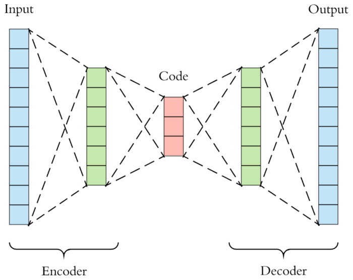
Image by Arden Dertat via Toward Data Science
The news which an autoencoder can be used for anomaly detection has been circulating on the internet for a while. Autoencoder was originally designed to learn the latent representation of a bunch of data. It consists of two parts, the encoder and decoder. Autoencoder will first encode the input data to a lower dimension of representation, it then decodes the representation back to its original form. Therefore, ones may suggest that if the difference between the reconstruction of a sample and its original form is big, then that sample could be an anomaly. Many internet articles suggested this idea, but only a few of them realised it. Therefore, I would like to implement this idea myself. By the way, Joseph Rocca wrote an exceptionally well introductory of autoencoders. If you are not familiar with the idea of an autoencoder, you are welcomed to read it.

Image by Riza Fahmi via Twitter.
The other reason I implemented this is that the data it used wasn’t audio-like or image-like data. We’ve seen so many successful stories of deep learning applying on image or audio data via end-to-end learning, i.e., without human-involved feature engineering. I wonder if a deep neural network can be applied on traditional table-like data as well. This paper used NetFlow data, which already discard much raw information of a packet. Furthermore, it grouped these NetFlow data with a specified time window and source IP then performed feature extraction on the grouped data. It would be interesting to see how a deep neural network performs on this kind of feature engineered data.
Feature Extraction
As mentioned in the paper, the authors first group the NetFlow records into 3-minute sliding windows based on the source IP address and compute the aggregated features. Here is the list of features extracted:
- mean and standard deviation of flow durations, number of packets, number of bytes, packet rate, and byte rate;
- entropy of protocol type, destination IP addresses, source ports, destination ports, and TCP flags; and
- proportion of ports used for common applications.
For the ports of common applications, as they didn’t mention which exact ports they chose, I selected these ports:- DHCP
- DNS
- FTP
- HTTP
- HTTPS
- IMAP
- IPSec
- LDAP
- NetBios
- NNTP
- NTP
- POP3
- RDP
- RPC
- SMTP
- SNMP
- SSH
- Telnet
- TFTP
- Other
The final number of features will be 69 instead of the original 53 (5 mean-related + 5 std-related + 5 entropy-related + 22 source-port-proportion + 22 dest-port-proportion).
I used PySpark to accelerate the extraction process.
1 | def extract_features(self) -> pyspark.sql.dataframe: |
Build Input for Model
This step is simple, I scaled the extracted with a min-max scaler, made all the values ranged from 0 to 1. Besides that, I also converted the data schema to Petastorm compatible schema. Petastorm enables our learning process directly applied to the data generated by big data processing platform, such as PySpark.
1 | def transform(self, remove_malicious=True, remove_null_label=True) -> pyspark.sql.DataFrame: |
Model
This paper used a VAE model (Variational autoencoder).
1 | class VAE(pl.LightningModule): |
Evaluation
Here comes the interesting part. We say that a sample is anomalous if its reconstruction error is big. Here lie two questions: how big is big, and how to compute the reconstruction error.
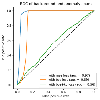
To compute the reconstruction error, instinctively, I would choose the same loss function from the model, which is binary cross-entropy with or without the regularisation term, the KL-divergence. However, neither of these are performing well. Before I started to give up, I used the L2 distance (MSE) as the reconstruction error. Boom! Surprisingly, it did a lot better the two previously mentioned loss.
Now we found the best way to compute reconstruction error. How do we decide the threshold? Let me plot the distribution of errors from normal and malicious samples.
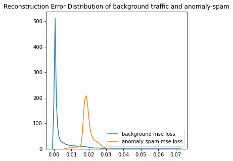
From the above image, we can see that the normal samples and malicious samples have two almost different error distribution, where the errors of the normal samples mostly concentrate at around 0.00, while the malicious ones concentrate at around 0.02. Based on the image, we can then set a hard threshold at 0.015. Balabit unsupervised wrote a detailed article on calibrating a threshold that may worth a read.
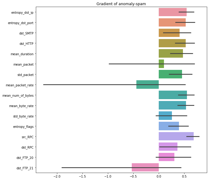
The authors also introduce a method to explain the VAE by the gradients. The explanation is somehow not very convincible, so I didn’t do a further experiment.
Code and Repo
Feel free to look on the codes. https://github.com/munhouiani/GEE