Byte-Pair Encoding

What is Byte-Pair Encoding

Byte-pair encoding (BPE) is a compression algorithm that can be used for text tokenization.

LLaMA 2 Open Foundation and Fine-Tuned Chat Models

📖 Abstract

In this work, we develop and release Llama 2, a collection of pretrained and fine-tuned large language models (LLMs) ranging in scale from 7 billion to 70 billion parameters. Our fine-tuned LLMs, called LLaMA 2-Chat are optimized for dialogue use cases. Our models outperform open-source chat models on most benchmarks we tested, and based on our human evaluations for helpfulness and safety, may be a suitable substitute for closedsource models. We provide a detailed description of our approach to fine-tuning and safety improvements of LLaMA 2-Chat in order to enable the community to build on our work and contribute to the responsible development of LLMs.

LLaMA Open and Efficient Foundation Language Models

📖 Abstract

We introduce LLaMA, a collection of foundation language models ranging from 7B to 65B parameters. We train our models on trillions of tokens, and show that it is possible to train state-of-the-art models using publicly available datasets exclusively, without resorting to proprietary and inaccessible datasets. In particular, LLaMA-13B outperforms GPT-3 (175B) on most benchmarks, and LLaMA65B is competitive with the best models, Chinchilla-70B and PaLM-540B. We release all our models to the research community.

Recall that from Off-Policy Gradient Methods, the objective function is

$$
\begin{aligned}
J^{\theta’}(\theta) &= \hat{\mathbb{E}} _{(s_t, a_t) \sim \pi _{\theta’} (\tau)} \bigg[ \frac{\pi _{\theta}(a_t | s_t)}{\pi _{\theta’}(a_t | s_t)} A^{\theta’}(s_t, a_t) \bigg]
\end{aligned}
$$

We learned that from Importance Sampling, the two distributions shouldn’t differ too much, therefore in PPO, they added a constraint term:

$$
J ^{\theta’} _{PPO} (\theta) = J ^{\theta’} (\theta) - \beta KL(\theta, \theta’)
$$

Where $\beta$ is a weight, this constraint term ensures that $\theta$ and $\theta’$ are similar.

Recall that from Policy Gradient Methods, the calculation of gradient is

$$
\begin{aligned}
\nabla \hat{R} _{\theta} &= \hat{ \mathbb{E}} _{\tau \sim \pi _{\theta}(\tau)} \bigg[ R(\tau) \nabla \log \pi _{\theta} (\tau) \bigg]
\end{aligned}
$$

where

• $\tau$ is a trajectory
• $\pi_{\theta}$ is a stochastic policy
• $\nabla_ {\pi _{\theta}}$ is the gradient operator of the policy $\pi$ with respect to $\theta$
• $\hat{\mathbb{E}} _{\tau \sim \pi _{\theta}(\tau)}[\dots]$ is the empirical average expectation over a finite batch of samples in an algorithm that alternates between sampling and optimization

In this setting, we have to:

• Use $\pi _{\theta}$ to collect data. When the parameter $\theta$ is updated, we must sample the training data again.
• This is called on-policy training

What Are Policy Gradient Methods

Policy gradient methods are a class of reinforcement learning algorithms used for optimizing parametrized policies by gradient descent to maximize the expected return, which is the cumulative reward received over a long-term horizon. These methods are based on updating the policy parameters such that the probabilities of actions leading to higher returns are increased. In comparison, the probabilities of actions leading to lower returns are decreased.

Iteratively optimizing the policy using this approach makes it possible to arrive at an optimal policy that maximizes the expected return. This technique has proven effective in solving complex decision-making problems in various fields, including robotics, game playing, and natural language processing.

Importance sampling is a technique commonly used in statistics and machine learning to estimate properties of a distribution that may be difficult to compute directly.

What is Out-of-Distribution (OOD) Detection and Why is it Important?

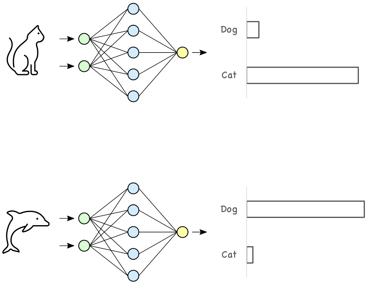
Most machine learning models are trained based on the closed-world assumption, meaning that the test data is assumed to have the same distribution as the training data. When we train a model, we usually form our training and testing data by randomly splitting the data we have into two sets, in which both datasets have the same label distribution. However, in the real-world scenario, this assumption doesn’t necessarily hold. For example, a model trained to classify cats and dogs may receive an image of a dolphin. Even worse, it might highly confident classify such inputs into in-distribution classes.

Detecting if the received model inputs have the same distribution as the training data is called out-of-distribution detection.

Stream-First Rendezvous Architecture

The rendezvous architecture was introduced by Ted Dunning in his book Machine Learning Logistics. This architecture is aimed to solve several real-world machine learning challenges:

• To meet large-scale changing data and changing goals.
• Isolation of models for evaluation in specifically customized, controlled environments.
• Managing multiple models in production at any given time.
• Have new models being readied to replace production models as situations change smoothly and without interruptions to service.

Gwern published a collection of Darknet Market Archives in 2015. While the dataset is comprehensive, a lot of works need to be done before we can start analyzing it. I put some effort to organize Gwern’s archives, extract only drug-related content, and construct a drug listing dataset in csv format.