Detecting Out-of-Distribution Samples with kNN
What is Out-of-Distribution (OOD) Detection and Why is it Important?
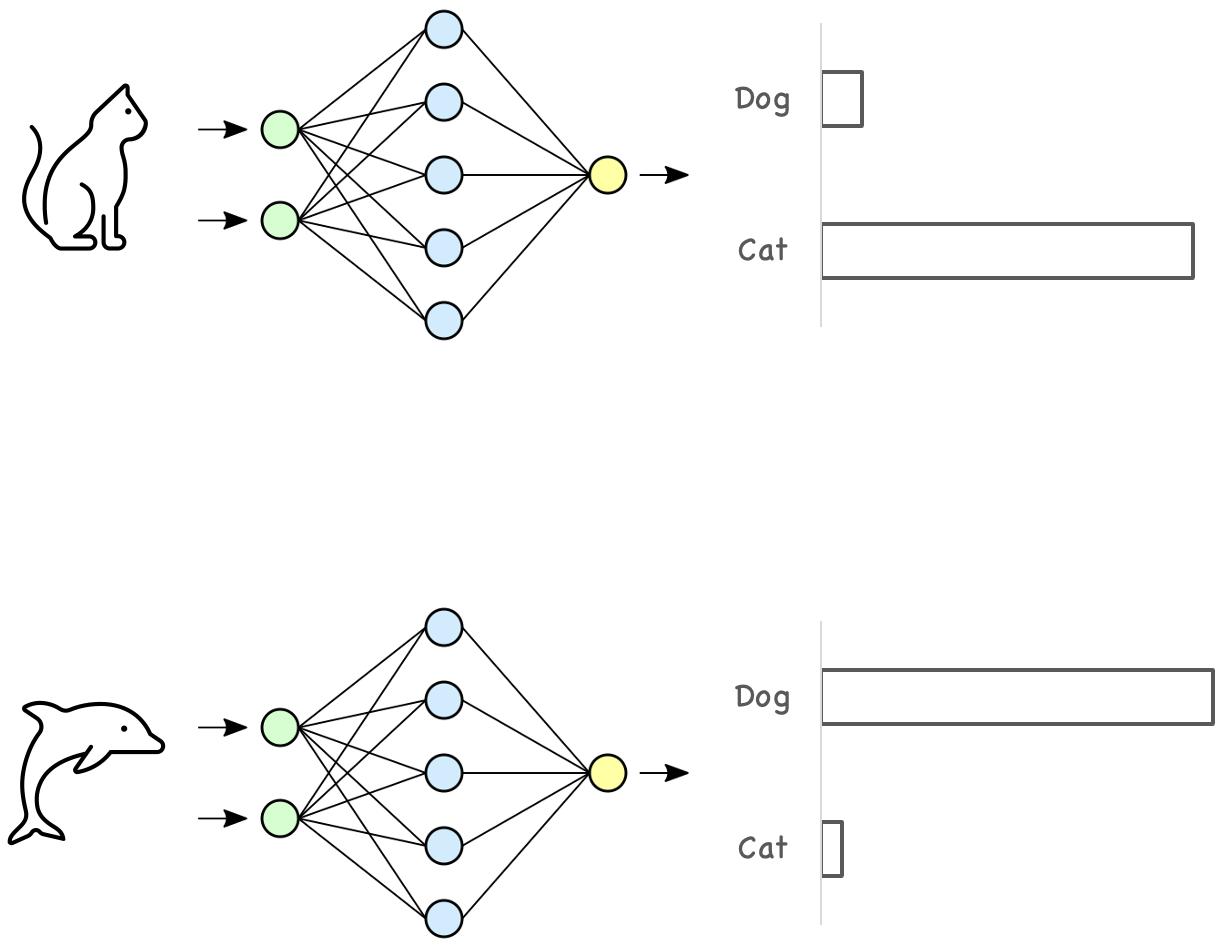
Most machine learning models are trained based on the closed-world assumption, meaning that the test data is assumed to have the same distribution as the training data. When we train a model, we usually form our training and testing data by randomly splitting the data we have into two sets, in which both datasets have the same label distribution. However, in the real-world scenario, this assumption doesn’t necessarily hold. For example, a model trained to classify cats and dogs may receive an image of a dolphin. Even worse, it might highly confident classify such inputs into in-distribution classes.
Detecting if the received model inputs have the same distribution as the training data is called out-of-distribution detection.
OOD detection plays a crucial part in modern-day machine learning services. For example, we can use the OOD detector as part of the machine learning operations to detect unknown inputs. When an unknown is seen, the machine learning service can safely reject the input instead of returning an answer from the model.
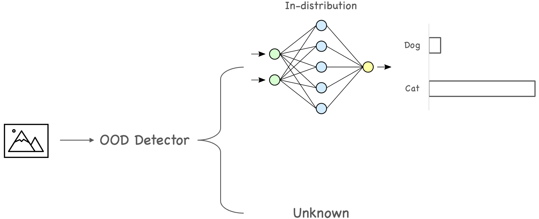
We can also use the result from an OOD detector as a filter for the data labeling task. For example, a machine learning service might receive a lot of inputs every day, and it is not feasible to let human labelers review all data. We can prioritize the process with an OOD detector by reviewing those out-of-distribution samples.
How is OOD Detection Methods Evaluted?
OOD detection can be seen as a binary classification problem. We often start by training a model with a dataset known as the in-distribution dataset, i.e., CIFAR-10. To evaluate an OOD detector, we will prepare another dataset not in the same domain as the training data, i.e., SHVN, known as the out-of-distribution dataset. We then combine these two datasets to check if the OOD detection knows which is from the in-distribution dataset and vice versa. We usually use label 1 (positive) for in-distribution and 0 (negative) for the out-distribution. Aside from the standard evaluation metrics, we also calculate the FP rate of the OOD detector when its TP rate is at 95%, denoted as FPR@TPR95.
OOD Detection Methods
From a comprehensive study by J. Yang et al., OOD detections methods can be categorized into:
- Classification methods
- Density-based methods
- Distance-based methods
- Reconstruction-based methods
Using kNN as an OOD Detector
The following sections are notes and implementation of a paper by Y. Sun et al.: Out-of-distribution detection with deep nearest neighbors.
Out-of-Distribution Detection for Single Feature
Before we dive into the kNN method, let’s see how out-of-distribution detection works on a single feature. For example, let’s say we have a feature $p$ that is normally distributed with a mean of $0$ and standard deviation of $1$, and $q$ is also drawn i.i.d. from the same distribution.
1 | import numpy as np |
We can use statistical distance measures, such as Wasserstein distance, to check if $p$ and $q$ have the same distribution. If they have the same distribution, the Wasserstein distance will be small. Otherwise, the resulting Wasserstein distance is large.
Traditional statistical distance measures are no longer applied to deep learning models because the inputs are very high-dimensional. Take a $32 \times 32$ color image as an example, its dimension is $32 \times 32 \times 3 = 3072$. Therefore, calculating statistical distance measures for all features is not feasible.
Core Idea: Embedding
Regarding deep learning models with high dimensional features, current OOD methods focus on the embedding space of a well-trained model. Distance-based methods assume that in the embedding space, OOD samples are relatively far away from in-distribution data. Density-based methods believe that in-distribution data follow certain probability distributions. Hence data falls into low-density regions are OOD.
However, these assumptions may not hold. Instead of imposing strong assumptions on the underlying embedding space, Y. Sun et al. use kNN, which is distributional assumption-free. Their algorithm is simple. First, they will gather distances of $k$-nearest neighbor of all in-distribution samples, then use those distances to determine a threshold. Any test data with a kNN distance larger than the threshold are flagged as OOD.
Train Resnet18 on CIFAR-10
We first train a ResNet18 model with CIFAR-10 data to demonstrate their approaches. This training code is slightly modified from the official Pytorch Lightning tutorial.
1 | class LitResnet(LightningModule): |
1 | model = LitResnet(lr=0.05, num_classes=10) |
This model achieves an accuracy of 94%.
Feature Extraction
We use the output of the last hidden layer (one layer before the output layer) as the features. Then, we normalize the features with the method described in the paper $\mathbf{z} = \phi(\mathbf{x}) / || \phi(\mathbf{x}) ||_{2}$.
1 | def extract_features(model, dataloader): |
1 | train_features = extract_features(model, train_loader) |
Find $k$-Nearest Neighbors with FAISS
We now need to find the distances of kNN and determine the threshold. First, we build an index using FAISS with the training features. Then we gather distances of $k$-th neighbors to the testing features. Here we set $k$ to 50. After that, we determine the threshold with 95% of TRP.
1 | # build index with training features |
Evaluate on OOD Data
We follow the same steps as above for the OOD data.
1 | # same as in-distribution data |
After getting the distances of $k$-th nearest neighbors of the OOD data, we can easily find the result by checking if the distance is greater than the threshold.
1 | tp = 0 |
The final result has an FPR@TPR95 of 37.45%, higher than the paper’s result of 24.53%. Developing an OOD detector depends on the quality of the model. The paper mentioned that we could improve the result by using contrastive learning. Contrastive learning helps bring data with the same label closer and push data with different labels further, which aligns with the usage of kNN.
Checkout the full notebook here: https://github.com/munhouiani/ood-knn
References
- J. Yang, K. Zhou, Y. Li, and Z. Liu, “Generalized out-of-distribution detection: A survey”, CoRR, vol. abs/2110.11334, 2021, [Online]. Available: https://arxiv.org/abs/2110.11334
- J. Ren and B. Lakshminarayanan, “Improving Out-of-Distribution Detection in Machine Learning Models”, Google Research Blog, Dec. 17, 2019. https://ai.googleblog.com/2019/12/improving-out-of-distribution-detection.html (accessed Dec. 02, 2022).
- Y. Sun, Y. Ming, X. Zhu, and Y. Li, “Out-of-distribution detection with deep nearest neighbors”, 2022.
- PL team, “PyTorch Lightning CIFAR10 ~94% Baseline Tutorial”, Pytorch Lightning, Apr. 28, 2022. https://pytorch-lightning.readthedocs.io/en/stable/notebooks/lightning_examples/cifar10-baseline.html (accessed Dec. 02, 2022).
- P. Mardziel, “Drift Metrics: How to Select the Right Metric to Analyze Drift”, Toward Data Science, Dec. 06, 2021. https://towardsdatascience.com/drift-metrics-how-to-select-the-right-metric-to-analyze-drift-24da63e497e (accessed Dec. 03, 2022).