Network Anomaly Detection with MIDAS, MIDAS-R, and MIDAS-F

Posted on 2021-03-27 Edited on 2023-08-15 Disqus:

Background

Anomaly detection has always been a challenging research field. An anomaly indicates a sudden and short-lived pattern change, while a detection algorithm aims to identify anomalies promptly. Detecting anomaly on networks levels up the problem as network monitoring devices usually collect data at high rates, which means a network anomaly detection algorithm should handle high-dimension, noisy, and massive data under power and communication constraints. We should also acknowledge that different anomalies exhibit themselves in network statistics in a different manner. A general anomaly detection model often does not exist. A model that detects surprising edges in a network is probably cannot detect micro cluster anomalies.

There are multiple ways to formulate a network anomaly detection problem. The simplest method is to calculate the mean and variance of any connection IP pairs and raise an alert once the connection count is away from 3 standard deviations of the means. This method holds an assumption: the connection count follows a Gaussian distribution. This assumption is strict and often false in a real-world situation.

Distribution of some connections

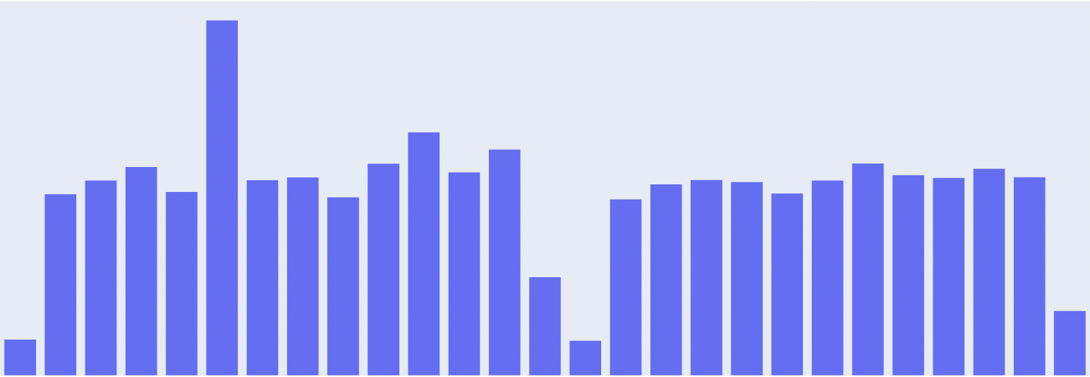
Pic 1. Distribution of connection counts from a real-world dataset, which is not a normal distribution.

Researchers had studied various machine learning approaches to this network anomaly detection problem. To represent a net flow, one either extracts hand-crafted features, such as ﬂow packet size, amount of specific signals, or build the representation automatically with deep neural networks, such as CNN. Afterwards, they either build an unsupervised model with an Isolation Forest, One-class SVM, or a Deep Autoencoder with these representations.

MIDAS authors formulated this problem differently. Instead of net flow, they model the network connections a graph, which kind of the networks’ nature. Their algorithm is a graph anomaly detection algorithm that works on a dynamic graph, a sweet capability where the current graph anomaly detection algorithms lack. Current graph algorithms only process a graph snapshot at specific intervals. They do not consider the temporal characteristics, in which everything happening at the current snapshot is somehow related to the past. Here are two graph snapshots from the same network at two different times. They are related to each other, yet their snapshots tell an entirely different story.

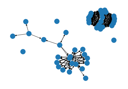Pic 2. Network Graph from Day 1

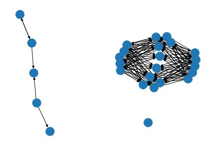Pic 3. Network Graph from Day 2

Properties of MIDAS

MIDAS has the following properties:

It can detect micro-cluster anomalies, which are suddenly arriving groups of suspiciously similar edge.
It processes each incoming edge within constant time and constant memory.

In general, MIDAS records the counts of every single edge with a Count-Min-Sketch data structure. Before we dive into their methodology, we should figure out what count-min-sketch is and why they use it.

Count-Min-Sketch (CMS)

We often use a hash map to maintain a counter:

1
2
3

d = {}

d[some_key] = d.get(some_key, 0) + 1

To retrieve the count of some_key, we use d[some_key]. This method does not scale as the number of keys in a hash map could be huge. Therefore, count-min-sketch (CMS) aims to serve as a frequency table that consumes only constant memory. In other words, the required memory of CMS does not increase when the number of keys increases.

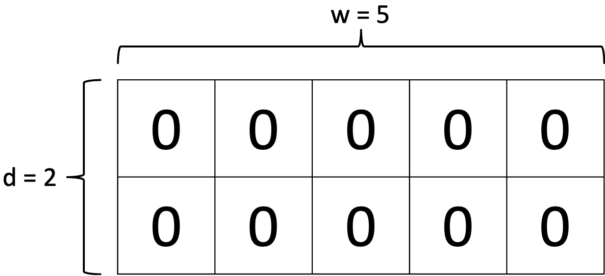
To use a CMS, we prepare $d$ different hash functions and the number of buckets of each hash function $w$. Then we initialise an matrix of size $d \times w$ with 0.

To update a count of some_key, we first hash some_key with a hash function $h_i$, and then increment the number at $cell(i, h_i(\text{some_key}))$. We continue this process until all $d$ hash functions have been used.

Of course, hash functions may conflict with each other due to the limited number of buckets. To retrieve the count of some_key, we get all counts of some_key from each row with $h_i(\text{some_key})$, then return the minimum value.

MIDAS

MIDAS will maintain two CMS, one for the total number of edges from $u$ to $v$ until the current time tick, denoted as $\hat{s} _{uv}$, and the number of edge from $u$ to $v$ at the current time tick, denoted as $\hat{a} _{uv}$. The time ticks mentioned here are discrete, for example, $t=10$. Since $\hat{a} _{uv}$ is used to count the edge from $u$ to $v$ at the current time tick, it will be reset every time MIDAS transition to the next time tick. For example, let us say we are at $t = 10$ and $\hat{a} _{uv} = 19$. Before we move to $t=11$, we will reset $\hat{a} _{uv}$ to $0$.

MIDAS assumes that the mean level (i.e. the average rate at which edges appear) in the current time tick (e.g. $t = 10$) is the same as the mean level before the current time tick ($t < 10$). Compare to the Gaussian mentioned we stated before, their assumption is weaker as they do not assume any distribution at each time tick.

With the chi-square goodness of fit test, they score any newly arriving edge $(u, v, t)$ with the following equation:

$$
score((u,v,t)) = (\hat{a} _{uv} - \frac{\hat{s} _{uv}}{t})^2 \frac{t^2}{\hat{s} _{uv}(t-1)}
$$

Let us walk through the proof one by one:

Proof

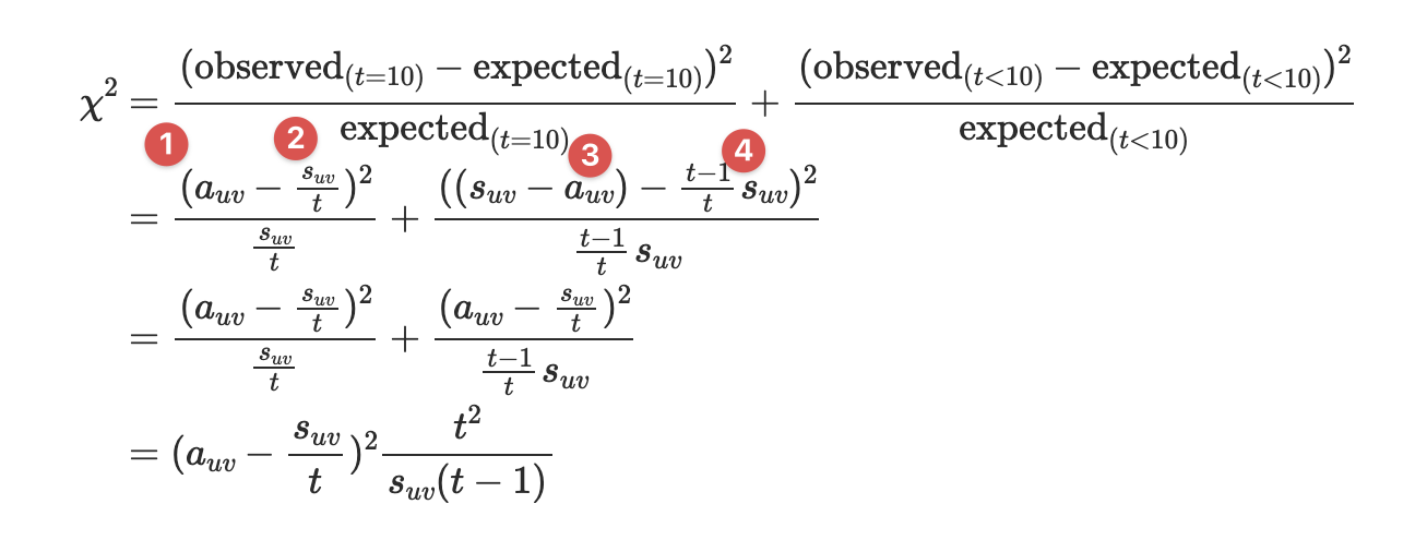
Recall that they have a CMS for the number of edge at the current time tick, therefore the observed count of edge $u \rightarrow v$ can be retrieved from $a_{uv}$.
Recall that they also have a CMS for the total number of edge until the current tick, therefore the mean level of edge $u \rightarrow v$ is calculated as $\frac{s_{uv}}{t}$.
To calculate the observed number of edge $u \rightarrow v$ before current time tick, we simply subtract $a_{uv}$ from $s_{uv}$.
Finally, to get the mean level of the number of edge $u \rightarrow v$ before current time tick, we calculate $\frac{t-1}{t} s_{uv}$.

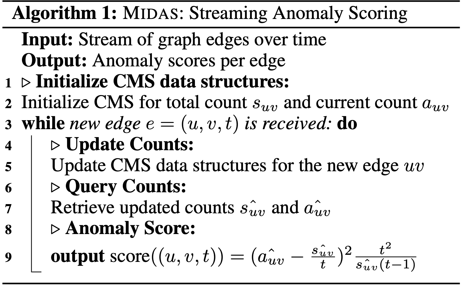
Here is the pseudocode of MIDAS:

MIDAS-R

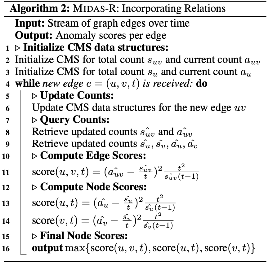
The “R” in MIDAS-R stands for “relations”. MIDAS-R aims to group related edges.

The first relation they incorporate is the temporal relation. Instead of resetting $a_{uv}$ before every transition, they reduce the count $a_{uv}$ by a fraction of $\alpha \in (0, 1)$. For example, let us say the $\alpha = 0.5$ and $a_{uv} = 20$. Before we transition to the next time tick, we reduce $a_{uv}$ to $10$ instead of resetting it to $0$.

DOS Attack

Besides temporal relations, MIDAS-R would also like to catch large groups of spatially nearby edges. Imagine there are lots of different hosts connected to the same machine A suddenly at $t=10$. MIDAS will probably not notice this anomaly as it scores the edges only. To tackle this problem, MIDAS-R creates four additional CMS structures, $a_u$, $s_u$, $a_v$, and $s_v$ to approximate the current and total edge counts adjacent to node $u$ and node $v$. Hence, for each incoming edge, MIDAS-R will compute three scores: one for edge $(u, v)$ as before, one for node $u$ and one for node $v$. Finally, it combines three scores by taking their maximum value.

Here is the pseudocode of MIDAS-R:

MIDAS-F

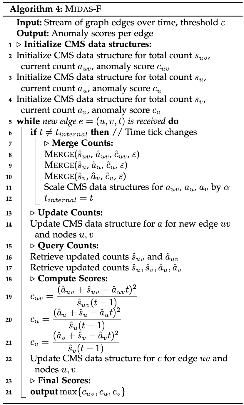
MIDAS and MIDAS-R are designed to update their records into their internal CMS structure immediately. Let us consider a DOS attack where many edges arrive within a brief period. At first, MIDAS can detect these anomalies. However, the mean level ($\frac{s_{uv}}{t-1}$) of the score increases as the attack continues, which leads to the increasing of the expected count of anomalous edge. Finally, MIDAS can no longer identify these anomalous edges.

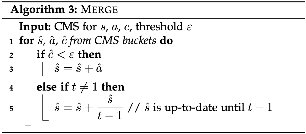
MIDAS-F introduces a conditional merge method to decide whether the current count $a$ should be merged into $s$ to prevent this poising effect. It uses another CMS structure $c _{uv}$ to keep track of the anomaly score. Whenever the time tick changes, if $c _{uv}$ is less than a pre-determined threshold $\epsilon$, the $a _{uv}$ will be added to $s _{uv}$. Otherwise, the expected count ($\frac{s _{uv}}{t-1}$) will be added to $s _{uv}$ to keep the mean level unchanged.

Here is the pseudocode of conditional merge:

MIDAS-F also redefined the $s_{uv}$ as the total number of edges from $u$ to $v$ until the previous time tick, not including the current edge count $a_{uv}$, leads to a minor change of scoring function:

$$
score(u, v, t) = \frac{(\hat{a} _{uv} + \hat{s} _{uv} - \hat{a} _{uv}t)^2}{\hat{s} _{uv}(t-1)}
$$

Here is the pseudocode of MIDAS-F:

MIDAS in Action

Before install, make sure you have Cmake >3.5.

To install MIDAS python, first clone this repo:

1	git clone https://github.com/munhouiani/MIDAS.git --branch v1.3.0 --recursive

Then change to the MIDAS directory and install:

1 2	cd MIDAS pip install .

I wrote an example of using MIDAS on real-word dataset here: MIDAS Example.ipynb

Conclusion

MIDAS is both a scalable and effective anomaly detection algorithm. There are several remaining problems we have to solve before deploying MIDAS into the production environment.

There are two needed thresholds in this algorithm. One is the $\epsilon$ in MIDAS-F, while the other one is to determine an instance is an anomaly or not. Unlike other supervised learning algorithms, where we usually set the threshold at 0.5, MIDAS’s score is unbounded. A systematic method to find thresholds is in need.

The other problem is whether we should update the MIDAS models. We know that a model drift phenomenon describes that the environment in which the model is operating is changing. A simple way to tackle the model drift problem is retraining our model periodically. MIDAS is an online learning algorithm by design, and we do not know yet if it is safe from the model drift problem.

References

[1] Real-Time Streaming Anomaly Detection in Dynamic Graphs

[2] Count-Min Sketch