From PPO to GDPO — Understanding the Evolution of Reinforcement Learning Algorithms
From PPO to GDPO — Understanding the Evolution of Reinforcement Learning Algorithms
Introduction: Why Reinforcement Learning?
The Two Stages of LLM Training
Training a Large Language Model is fundamentally a two-stage process:
Stage 1: Pre-training (Knowledge Acquisition)
- The model learns from trillions of tokens of text
- It learns to predict the next token: $P(x_t | x_{<t})$
- Result: A “document completor” that understands language structure
Stage 2: Post-training (Behavioral Alignment)
- The model learns to be helpful, harmless, and honest
- It learns to follow instructions and provide useful responses
- Result: A helpful AI assistant
The Problem: A pre-trained model asked “How do I bake a cake?” might respond with “How do I bake a pie?” — continuing a pattern rather than answering the question.
Why Not Just Use Supervised Fine-Tuning?
Supervised Fine-Tuning (SFT) teaches the model to mimic expert responses. While effective for basic tasks, it has critical limitations:
| Limitation | Description |
|---|---|
| Data Ceiling | Limited by availability of expert demonstrations |
| Mimicry Problem | Model copies style without understanding reasoning |
| No Negative Feedback | Model is told what to do, but rarely what not to do |
| No Exploration | Cannot discover novel solutions beyond training data |
The RL Solution
Reinforcement Learning solves these problems by defining the goal (what we want) without specifying the path (how to get there):
1 | Instead of: "Here's the perfect poem, copy it" |
This enables:
- Trial and Error: Model can explore and discover novel solutions
- Negative Feedback: Low scores teach what to avoid
- Emergent Behaviors: Self-correction, extended thinking, “aha moments”
Theoretical Foundations
The Language Model as an Agent
To understand RL for LLMs, we must map text generation onto the Markov Decision Process (MDP) framework:
| MDP Component | In LLM Context |
|---|---|
| State ($s_t$) | The prompt + all tokens generated so far |
| Action ($a_t$) | Selecting the next token from vocabulary (32K-100K options) |
| Transition ($P$) | Deterministic: “The cat sat on” + “mat” → “The cat sat on mat” |
| Reward ($R$) | Score from reward model or verifier (e.g., 1 for correct, 0 for wrong) |
| Policy ($\pi_\theta$) | The LLM itself — outputs probability distribution over tokens |
The Optimization Objective
The goal is to maximize expected cumulative reward:
$$J(\theta) = \mathbb{E}_{\tau \sim \pi_\theta} \left[ \sum_{t=0}^{T} \gamma^t r_t \right]$$
Where:
- $\tau$ = trajectory (complete sequence of tokens)
- $\gamma$ = discount factor (typically close to 1 for LLMs)
- $r_t$ = reward at timestep $t$
The Policy Gradient Theorem
Since we cannot differentiate through the discrete sampling of tokens, we use the Policy Gradient:
$$\nabla_\theta J(\theta) = \mathbb{E}_{\tau \sim \pi_\theta} \left[ \sum_t \nabla_\theta \log \pi_\theta(a_t|s_t) \cdot A^{\pi}(s_t, a_t) \right]$$
The Advantage Function $A^{\pi}(s_t, a_t)$ is crucial — it answers:
“How much better was this specific action compared to the average action I could have taken?”
$$A^{\pi}(s_t, a_t) = Q^{\pi}(s_t, a_t) - V^{\pi}(s_t)$$
Where:
- $V^{\pi}(s_t)$ = Value Function (state-value): “If I’m in state $s_t$, what’s my expected total future reward?”
- In LLM terms: “Given the prompt + tokens so far, how good is my situation on average?”
- This is what the Critic network learns to predict in PPO
- $Q^{\pi}(s_t, a_t)$ = Q-Function (action-value): “If I’m in state $s_t$ AND I take action $a_t$, what’s my expected total future reward?”
- In LLM terms: “Given the prompt + tokens so far, if I choose this specific next token, how good will my final answer be?”
Intuition: $V$ tells you “how good is your current position on average” while $Q$ tells you “how good is your current position if you take this specific action.” The difference ($Q - V$) tells you whether this particular action is better or worse than your average option — that’s the Advantage.
The history of LLM alignment is essentially the history of finding better, cheaper, and more stable ways to estimate this Advantage function.
PPO: The Foundation
Origin and Purpose
Proximal Policy Optimization (PPO) was introduced by Schulman et al. at OpenAI in 2017. It was the algorithm that proved RLHF could scale to billions of parameters, powering:
- InstructGPT
- Early GPT-4
- ChatGPT’s initial alignment
The Problem PPO Solves: Policy Collapse
In standard policy gradient methods, if an update is too large, the policy can change drastically. This leads to:
- Policy Collapse: The model enters a bad region of parameter space
- Catastrophic Forgetting: Good behaviors are lost
- Training Instability: Rewards oscillate wildly
PPO enforces a Trust Region — limiting how much the policy can change in a single update.
The Four-Model Architecture
PPO requires maintaining four neural networks simultaneously:
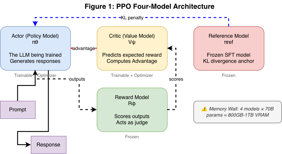
Figure 1: The PPO architecture requires four neural networks: Actor (policy model being trained), Critic (value model predicting expected reward), Reference (frozen SFT model for KL constraint), and Reward Model (scoring outputs). This creates the “memory wall” problem for large models.
| Model | Role | Memory Cost |
|---|---|---|
| Actor ($\pi_\theta$) | The LLM being trained | Trainable + Optimizer States |
| Critic ($V_\phi$) | Predicts expected future reward | Trainable + Optimizer States |
| Reference ($\pi_{ref}$) | Frozen SFT model for KL constraint | Frozen weights |
| Reward ($R_\psi$) | Scores the Actor’s outputs | Frozen weights |
The Memory Wall: For a 70B model, this setup requires ~800GB-1TB of VRAM, necessitating massive GPU clusters.
Common Confusion: Critic vs Reward Model
Both the Critic and Reward Model output a “score,” which often confuses newcomers. The key difference is when they act and what they represent:
| Model | When It Acts | What It Does | Role |
|---|---|---|---|
| Reward Model | After generation is complete | Looks at finished answer, gives final grade (e.g., “Correct: +1”) | Ground Truth — the actual goal |
| Critic | Before/during generation | Looks at current state, predicts “I expect to score 0.7 on this” | Baseline/Expectation — used for normalization |
Why do we need both? To calculate the Advantage (how much better/worse than expected):
$$\text{Advantage} = \text{Actual Reward (from Reward Model)} - \text{Expected Reward (from Critic)}$$
- If you get 0.8, but Critic expected 0.9 → Negative advantage (worse than expected)
- If you get 0.8, but Critic expected 0.2 → Large positive advantage (much better than expected)
The Critic normalizes the reward signal so the model knows if an action was truly “special” or just “average.” This is exactly what GRPO replaces with group statistics.
The PPO Objective Function
PPO uses a “clipped surrogate” objective to ensure stability:
Step 1: Calculate the Probability Ratio
$$r_t(\theta) = \frac{\pi_\theta(a_t|s_t)}{\pi_{old}(a_t|s_t)}$$
- If $r_t > 1$: action is more likely now than before
- If $r_t < 1$: action is less likely
Step 2: Calculate Advantage using GAE
The Critic computes the advantage via Generalized Advantage Estimation (GAE).
What is GAE? When calculating the Advantage ($A = Q - V$), we face a tradeoff:
- One-step estimate ($A = r_t + \gamma V(s_{t+1}) - V(s_t)$): Low bias, high variance — uses actual reward but noisy
- Multi-step estimate: Look further ahead for more signal, but compounds errors from the Critic
GAE solves this by computing a weighted average of all possible n-step estimates:
$$\hat{A}_t^{GAE} = \sum_{l=0}^{\infty} (\gamma \lambda)^l \delta_{t+l}$$
Where $\delta_t = r_t + \gamma V(s_{t+1}) - V(s_t)$ is the one-step TD error, and $\lambda \in [0, 1]$ controls the tradeoff:
- $\lambda = 0$: Pure one-step (high variance, low bias)
- $\lambda = 1$: Full Monte Carlo (low variance, high bias)
- $\lambda = 0.95$: Typical setting — balanced
In LLM terms: GAE helps the model understand “was this token choice good?” by looking not just at the immediate effect, but also at how the rest of the response turned out — while discounting increasingly uncertain future predictions.
Result of GAE:
- Positive Advantage: Model did better than expected → Increase probability
- Negative Advantage: Model did worse than expected → Decrease probability
Step 3: Apply Clipping
$$L^{CLIP}(\theta) = \mathbb{E}_t \left[ \min(r_t(\theta)\hat{A}_t, \text{clip}(r_t(\theta), 1-\epsilon, 1+\epsilon)\hat{A}_t) \right]$$
The clip bounds (typically $\epsilon = 0.2$) limit the ratio to $[0.8, 1.2]$:
- Updates cannot push probability too high or too low
- Creates a “safe zone” for stable training
Why PPO Failed for Modern Reasoning
| Problem | Description |
|---|---|
| Memory Cost | 4 models × 70B = prohibitive VRAM requirements |
| Critic Instability | Hard to predict value of intermediate reasoning steps |
| Hyperparameter Sensitivity | Small changes cause training collapse |
| Sparse Rewards | Binary pass/fail makes credit assignment difficult |
These limitations drove the search for alternatives.
DPO: The Offline Revolution
The Key Insight
In 2023, researchers at Stanford asked a fundamental question:
“If we have preference data (Response A is better than Response B), do we really need a separate Reward Model and Critic?”
The answer was no. DPO (Direct Preference Optimization) exploits a mathematical duality:
- For every reward function, there exists a unique optimal policy
- We can optimize the policy directly on preference pairs
What Changed: From Online to Offline
| Aspect | PPO (Online) | DPO (Offline) |
|---|---|---|
| Data | Generated during training | Pre-collected preference pairs |
| Models | 4 (Actor, Critic, Ref, Reward) | 2 (Actor, Reference) |
| Training Loop | Generate → Score → Update | Load pairs → Update |
| Exploration | Yes (generates new samples) | No (fixed dataset) |
The DPO Objective
Given preference pairs $(y_w, y_l)$ where $y_w$ is preferred over $y_l$:
$$L_{DPO} = -\mathbb{E}_{(x, y_w, y_l)} \left[ \log \sigma \left( \beta \log \frac{\pi_\theta(y_w|x)}{\pi_{ref}(y_w|x)} - \beta \log \frac{\pi_\theta(y_l|x)}{\pi_{ref}(y_l|x)} \right) \right]$$
Breaking it down:
- $\frac{\pi_\theta(y|x)}{\pi_{ref}(y|x)}$ = How much has the model deviated from reference?
- DPO wants to increase this ratio for winners, decrease for losers
- $\beta$ = Temperature controlling how strongly we enforce KL constraint
- $\sigma$ = Sigmoid function (turns into classification)
DPO Variants
| Variant | Description |
|---|---|
| Offline DPO | Standard: train once on fixed dataset |
| Iterative DPO | Cyclical: generate new pairs → label → retrain |
| Online DPO | Like PPO: generate during training, immediate labeling |
Why DPO Failed for Reasoning
While DPO revolutionized chat alignment (style, safety, helpfulness), it hit a hard ceiling for reasoning tasks:
| Problem | Explanation |
|---|---|
| Out-of-Distribution | Can only learn from provided solutions, cannot explore |
| Copycat Effect | Mimics form of correct answer without understanding process |
| No Trial-and-Error | Cannot generate, verify, and learn from own attempts |
| Static Data | Hard problems need model to discover novel reasoning paths |
The Fundamental Tension: Reasoning needs online exploration (like PPO), but PPO’s memory cost was prohibitive. This tension birthed GRPO.
GRPO: The Reasoning Renaissance
Origin: DeepSeek-Math and DeepSeek-R1
In early 2024, DeepSeek AI introduced Group Relative Policy Optimization (GRPO) in their paper “DeepSeekMath: Pushing the Limits of Mathematical Reasoning.” This algorithm enabled:
- DeepSeek-R1’s breakthrough reasoning capabilities
- “Aha moments” and emergent self-correction
- Training massive reasoning models on accessible hardware
The Core Innovation: Killing the Critic
GRPO’s insight: The Critic in PPO is just estimating a baseline. Why train a neural network when we can calculate it directly?
| PPO Approach | GRPO Approach |
|---|---|
| Train Critic to predict $V(s)$ | Sample G outputs, use group mean |
| Compare to neural network prediction | Compare to other outputs from same model |
| Memory: 4 models | Memory: 2 models |
The Classroom Analogy
PPO:
- Student answers a question
- Teacher (Reward Model) grades it
- Statistician (Critic) predicts what grade should have been
- Student learns from the difference
GRPO:
- Teacher asks a question
- Student writes 64 different answers
- Teacher grades all 64
- Student learns to favor above-average answers, avoid below-average
How GRPO Works
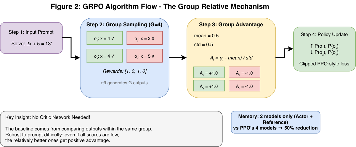
Figure 2: The GRPO algorithm flow shows how the model generates G outputs for each prompt, scores them, calculates group-relative advantages using mean/std normalization, and updates the policy to favor above-average outputs. No Critic network is needed.
Step 1: Group Sampling
For each prompt $q$, generate G outputs ${o_1, o_2, …, o_G}$ (typically G = 16-64)
Step 2: Scoring
Use reward model or rule-based verifier to score all outputs: ${r_1, r_2, …, r_G}$
Step 3: Advantage Calculation
Normalize each reward against group statistics:
$$A_i = \frac{r_i - \text{mean}({r_1, …, r_G})}{\text{std}({r_1, …, r_G}) + \epsilon}$$
Why this works:
- If all answers are bad (scores 0.1, 0.2, 0.1), the 0.2 still gets positive advantage
- If all answers are good (scores 0.9, 0.9, 0.8), the 0.8 gets negative advantage
- Algorithm is robust to prompt difficulty
Step 4: Policy Optimization
Update weights to maximize likelihood of high-advantage outputs, with KL constraint.
The “Aha Moment” Phenomenon
During training of DeepSeek-R1-Zero, researchers observed emergent behaviors that were not explicitly programmed:
| Behavior | Description |
|---|---|
| Self-Correction | “Wait, this assumes X which is wrong. Let me try Y…” |
| Extended Thinking | Response length grew from hundreds to thousands of tokens |
| Phase Transitions | Sudden jumps in benchmark scores (“aha moments”) |
These behaviors prove that online RL with GRPO unlocks capabilities that SFT and DPO cannot — the model discovers strategies humans might not know how to demonstrate.
GRPO vs PPO Comparison
| Feature | PPO | GRPO |
|---|---|---|
| Model Count | 4 (Actor, Ref, Reward, Critic) | 2 (Actor, Ref) + Group Buffer |
| Memory | ~4x model size | ~2x model size |
| Advantage Source | Neural Network (Critic) | Group Statistics (Mean/Std) |
| Compute Overhead | Forward/backward on Critic | Generating G samples |
| Reward Signal | Absolute | Relative |
| Best For | General chat, short tasks | Reasoning, math, coding |
Advanced Algorithms: GRPO+, DAPO, and GDPO
The Problems with Basic GRPO
While GRPO solved the memory bottleneck, researchers identified several failure modes:
| Problem | Description |
|---|---|
| Entropy Collapse | Model converges to single “safe” pattern, stops exploring |
| Gradient Deadzones | All-correct or all-wrong batches produce zero gradient |
| Multi-Objective Blindness | Summed rewards mask individual signal contributions |
| Length Bias | Long responses dilute gradient signal |
Deep Dive: What is Entropy Collapse?
Entropy in this context measures the uncertainty or randomness of the model’s token choices:
- High Entropy: Model assigns similar probabilities to many tokens → exploring diverse options
- Low Entropy: Model puts ~100% probability on one token → exploiting what it knows
The Vicious Cycle of Collapse:
- Discovery: Model tries a phrase (e.g., “Step 1:”) and happens to get a positive reward
- Reinforcement: Algorithm increases probability of that pattern
- Loss of Diversity: That pattern is now more likely, so model samples it more often
- Feedback Loop: Since it’s sampled more, it gets rewarded more (if still “safe”)
- Collapse: Probability distribution transforms from a gentle hill (diverse) to a sharp spike (single option)
Why This Fails for Reasoning:
Imagine a student who learns that writing “The answer is 5” gets partial credit. With entropy collapse, they stop trying to solve equations — they just write “The answer is 5” on every question because it’s the “safest” bet they know. They are stuck in a local optimum (okay, but not optimal).
When given a difficult problem requiring a creative approach, a collapsed model produces a “safe” but likely incorrect answer. It stops “thinking” and starts “reciting.”
GRPO+
GRPO+ was developed for the DeepCoder model and addresses entropy collapse:
Innovation 1: Remove KL Divergence (and the Reference Model)
- Standard RLHF keeps model close to SFT baseline via KL penalty
- For reasoning, SFT baseline doesn’t know how to “think”
- GRPO+ sets $\beta_{KL} = 0$ to allow radical policy shifts
Memory Implication: When $\beta_{KL} = 0$, the Reference Model serves no purpose and can be removed entirely. This further reduces VRAM usage from 2 models to effectively 1 model (just the Actor), enabling even larger batch sizes or model scales. DeepSeek-R1-Zero leveraged this to train without any SFT anchor.
Why Remove KL Divergence? The “Leash” Analogy
Think of KL divergence as a leash attached to your dog (the policy):
| With Leash (KL Penalty) | Without Leash (β=0) |
|---|---|
| Dog can explore, but only within leash radius | Dog can run anywhere in the park |
| Safe: won’t run into traffic | Risky: might find trouble, but also treasure |
| Predictable: stays near you (SFT baseline) | Unpredictable: discovers new behaviors |
For general chat: Keep the leash. You want responses similar to your carefully curated SFT data. Going too far from the baseline risks incoherence or harmful outputs.
For reasoning/math: Remove the leash. Your SFT model doesn’t know how to “think through” hard problems — it was trained on direct answers. You want the model to discover entirely new reasoning patterns, even if they look nothing like the original distribution.
This is why models like DeepSeek-R1-Zero can develop emergent reasoning behaviors (chain-of-thought, self-verification) that weren’t in the training data — they weren’t constrained to stay near a baseline that didn’t have these skills.
Innovation 2: Asymmetric Clipping
1 | # Standard GRPO: symmetric clipping |
Why Asymmetric?
- Conservative lower bound (0.8): Don’t destroy knowledge
- Aggressive upper bound (1.28): Encourage discovery of good actions
- Result: Maintains exploration (entropy) much longer
Innovation 3: Iterative Context Lengthening
- Start with short contexts (4K tokens)
- Gradually increase (16K → 32K) as training stabilizes
- Prevents model from getting lost in “hallucinated ramblings”
DAPO: Decoupled Clip and Dynamic Sampling
DAPO (2025) represents the current state-of-the-art, specifically designed to beat DeepSeek-R1-Zero on AIME benchmarks.
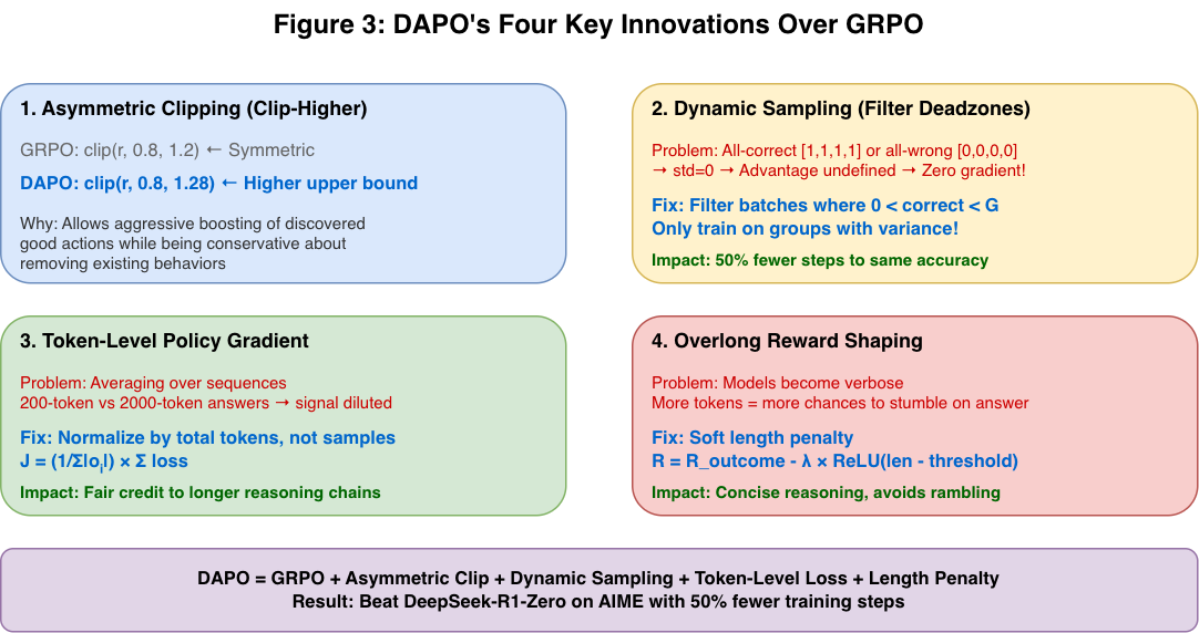
Figure 3: DAPO introduces four key improvements over GRPO: (1) Asymmetric clipping for better exploration, (2) Dynamic sampling to filter uninformative batches, (3) Token-level loss normalization, and (4) Overlong reward shaping to prevent verbosity.
Innovation 1: Asymmetric Clipping (Clip-Higher)
Same as GRPO+ — uses different bounds for increase vs decrease:
1 | def dapo_clip(ratio, advantages, eps_low=0.2, eps_high=0.28): |
Innovation 2: Dynamic Sampling
The “gradient deadzone” problem:
| Scenario | Rewards | Mean | Std | Advantage |
|---|---|---|---|---|
| Too Easy | [1, 1, 1, 1] | 1 | 0 | 0/0 = undefined |
| Too Hard | [0, 0, 0, 0] | 0 | 0 | 0/0 = undefined |
DAPO’s Solution: Filter batches that provide no learning signal.
1 | def dynamic_sampling_rollout(self, dataloader): |
Impact: Every training step provides meaningful gradient. DAPO converges to higher accuracy with 50% fewer training steps.
Connection to Active Learning: Dynamic Sampling is essentially a form of uncertainty-based active learning. By filtering for groups where the model shows variance (some correct, some incorrect), DAPO automatically focuses compute on problems in the model’s “Zone of Proximal Development” — problems it’s uncertain about and can learn from. This is analogous to curriculum learning, but discovered dynamically rather than pre-specified.
Innovation 3: Token-Level Policy Gradient
Standard methods average loss over sequences. For long Chain-of-Thought:
- 200-token answer vs 2000-token answer
- Averaging dilutes the signal for longer (often more rigorous) reasoning
DAPO: Normalize by total tokens, not number of samples:
$$J_{DAPO} = \frac{1}{\sum |o_i|} \sum_{i,t} \text{loss}_{i,t}$$
Innovation 4: Overlong Reward Shaping
Reasoning models tend toward verbosity (more tokens = more chances to be right). DAPO adds a soft length penalty:
$$R_{final} = R_{outcome} - \lambda \cdot \text{ReLU}(\text{length} - L_{threshold})$$
GDPO: Group Reward-Decoupled Normalization Policy Optimization
GDPO (Group reward-Decoupled Normalization Policy Optimization) addresses a critical problem that GRPO and DAPO don’t solve: multi-objective optimization where you need to balance multiple, potentially conflicting reward signals.
The Reward Signal Collapse Problem
In real-world alignment, we rarely optimize a single metric. We want:
- Correctness (is the answer right?)
- Formatting (is it valid JSON/markdown?)
- Safety (does it avoid harmful content?)
- Brevity (is it concise?)
Standard GRPO aggregates these into a scalar before calculating advantage:
$$R_{total} = w_A R_{correctness} + w_B R_{format} + w_C R_{safety} + …$$
This causes Reward Signal Collapse. Consider this scenario:
| Output | Correctness ($R_c$) | Format ($R_f$) | Total |
|---|---|---|---|
| $\tau_1$ | 1 (correct) | 0 (bad JSON) | 1 |
| $\tau_2$ | 0 (wrong) | 1 (good JSON) | 1 |
In standard GRPO:
- Rewards = {1, 1}
- Mean = 1, Std = 0
- Advantage = $(1-1)/0$ = undefined
Even with more samples, $\tau_1$ and $\tau_2$ get identical advantages. The model cannot learn that “Correctness is good” independently of “Formatting is good” — it becomes confused, unable to disentangle which feature caused the reward.
The GDPO Algorithm: Normalize First, Aggregate Second
⚠️ Common Misconception: Weighted aggregation of rewards is NOT new to GDPO. GRPO and DAPO also use weighted sums like $R = w_1 R_1 + w_2 R_2 + …$.
What IS new: The order of operations. GRPO does “Sum → Normalize” while GDPO does “Normalize → Sum”. This seemingly small change completely solves the reward signal collapse problem.
GDPO inverts the order of operations: instead of normalizing the sum, it normalizes each component independently.
Step-by-Step GDPO Execution:
- Group Generation: Sample $G$ outputs ${o_1, …, o_G}$ for prompt $x$
- Multi-Objective Evaluation: Compute reward vector $\mathbf{r}_i = [r_{i,1}, r_{i,2}, …, r_{i,K}]$ for each output
- Component-wise Normalization: For each objective $k$:
- Calculate group mean: $\mu_k = \frac{1}{G} \sum_{i=1}^G r_{i,k}$
- Calculate group std: $\sigma_k = \sqrt{\frac{1}{G} \sum_{i=1}^G (r_{i,k} - \mu_k)^2}$
- Compute normalized advantage: $\hat{A}_{i,k} = \frac{r_{i,k} - \mu_k}{\sigma_k + \epsilon}$
- Weighted Aggregation: $A_i^{GDPO} = \sum_{k=1}^K w_k \hat{A}_{i,k}$
- Global Normalization (optional): Normalize final advantages across batch
Worked Example: Computing GDPO Z-Scores Step-by-Step
🔑 Key Insight: The normalized advantage $\hat{A}$ is a Z-score — it tells you “how many standard deviations away from the group mean is this sample?” This is NOT the raw reward value!
Scenario: Tool calling task with 4 outputs in a group
| Output | Tool Choice ($R_t$) | JSON Format ($R_j$) |
|---|---|---|
| $\tau_1$ | 1 (correct tool) | 0 (invalid JSON) |
| $\tau_2$ | 1 (correct tool) | 1 (valid JSON) |
| $\tau_3$ | 0 (wrong tool) | 1 (valid JSON) |
| $\tau_4$ | 0 (wrong tool) | 0 (invalid JSON) |
Step 1: Compute statistics for Tool Choice ($R_t$)
- Raw values: [1, 1, 0, 0]
- Mean: $\mu_t = (1+1+0+0)/4 = 0.5$
- Standard deviation: $\sigma_t = \sqrt{((1-0.5)^2 + (1-0.5)^2 + (0-0.5)^2 + (0-0.5)^2)/4} = \sqrt{0.25} = 0.5$
Step 2: Compute Z-scores for Tool Choice
- $\hat{A}_{1,t} = (1 - 0.5) / 0.5 = +1.0$ ← “1 std above mean”
- $\hat{A}_{2,t} = (1 - 0.5) / 0.5 = +1.0$
- $\hat{A}_{3,t} = (0 - 0.5) / 0.5 = -1.0$ ← “1 std below mean”
- $\hat{A}_{4,t} = (0 - 0.5) / 0.5 = -1.0$
Step 3: Compute statistics for JSON Format ($R_j$)
- Raw values: [0, 1, 1, 0]
- Mean: $\mu_j = 0.5$, Std: $\sigma_j = 0.5$
Step 4: Compute Z-scores for JSON Format
- $\hat{A}_{1,j} = (0 - 0.5) / 0.5 = -1.0$
- $\hat{A}_{2,j} = (1 - 0.5) / 0.5 = +1.0$
- $\hat{A}_{3,j} = (1 - 0.5) / 0.5 = +1.0$
- $\hat{A}_{4,j} = (0 - 0.5) / 0.5 = -1.0$
Step 5: Aggregate with weights (using $w_t = 1, w_j = 1$)
| Output | $\hat{A}_t$ (Z-score) | $\hat{A}_j$ (Z-score) | $A^{GDPO} = \hat{A}_t + \hat{A}_j$ |
|---|---|---|---|
| $\tau_1$ | +1.0 | -1.0 | 0 (good tool, bad format) |
| $\tau_2$ | +1.0 | +1.0 | +2 (good at both!) |
| $\tau_3$ | -1.0 | +1.0 | 0 (bad tool, good format) |
| $\tau_4$ | -1.0 | -1.0 | -2 (bad at both) |
Result: The model receives clear, disentangled feedback:
- $\tau_2$ gets strongly reinforced (excellent at both)
- $\tau_4$ gets strongly discouraged (poor at both)
- $\tau_1$ and $\tau_3$ get neutral signal — they’re not wrong overall, just have different strengths
❌ Common Mistake: Using raw rewards instead of Z-scores. If you computed $A_1 = R_t + R_j = 1 + 0 = 1$ instead of using Z-scores, you’d get wrong gradients!
Now consider a more realistic scenario with heterogeneous reward distributions:
| Output | Safety ($R_s$) | Conciseness ($R_l$) |
|---|---|---|
| $\tau_1$ | 0 (safe) | 0.3 (verbose) |
| $\tau_2$ | -100 (unsafe) | 0.9 (concise) |
| $\tau_3$ | 0 (safe) | 0.7 (moderate) |
In GRPO (summed first):
- The massive -100 spike dominates variance
- Safe but verbose ($\tau_1$) and safe but moderate ($\tau_3$) look similar after normalization
- The conciseness signal is drowned out
In GDPO (normalized per-component):
- Safety normalized: $\tau_1, \tau_3$ get similar positive scores, $\tau_2$ gets large negative
- Conciseness normalized independently: $\tau_2$ gets +1, $\tau_3$ gets moderate, $\tau_1$ gets -1
- Final gradient: “Be Safe AND Be Concise” — signals preserved
GDPO Empirical Results
| Task | GRPO Performance | GDPO Performance | Improvement |
|---|---|---|---|
| Math + Length Constraint | Baseline | +6.3% accuracy | Length violations reduced 80% |
| Tool Calling (Choice + Format) | 90% choice, 60% format | 92% choice, 95% format | Format massively improved |
| Code + Safety | Safety often ignored | Both optimized | Clear multi-objective signal |
When to Use GDPO
Use GDPO when:
- You have multiple, potentially conflicting reward signals
- You observe “Reward Hacking” where the model ignores one objective to maximize another
- You are building agentic systems with complex tool-use constraints
- Your rewards have different scales or distributions (binary vs continuous, sparse vs dense)
GDPO vs DAPO: DAPO focuses on single-objective efficiency (dynamic sampling, asymmetric clipping). GDPO focuses on multi-objective clarity. In practice, you can combine them: use GDPO’s decoupled normalization with DAPO’s dynamic sampling and asymmetric clipping.
Comparative Analysis
Algorithm Comparison Table
| Feature | PPO | DPO | GRPO | GRPO+ | DAPO | GDPO |
|---|---|---|---|---|---|---|
| Type | Online Actor-Critic | Offline | Online Policy-Gradient | Online | Online | Online |
| Models Required | 4 | 2 | 2 | 2 | 2 | 2 |
| Memory Cost | Very High | Low | Low | Low | Low | Low |
| Baseline | Learned Critic | Implicit | Group Mean | Group Mean | Filtered Group Mean | Per-Reward Mean |
| Reward Handling | Single Scalar | Pairwise Preference | Summed Scalar | Summed Scalar | Summed + Length Penalty | Decoupled Multi-Reward |
| Clipping | Symmetric | None | Symmetric | Asymmetric | Asymmetric | Symmetric |
| Best For | General Chat | Style/Safety | Math/Code | Code | Advanced Reasoning | Multi-Objective Agentic |
| Key Innovation | Trust Region | Implicit Reward | Critic-Free | KL-Free | Dynamic Sampling | Per-Reward Normalization |
Evolution Diagram
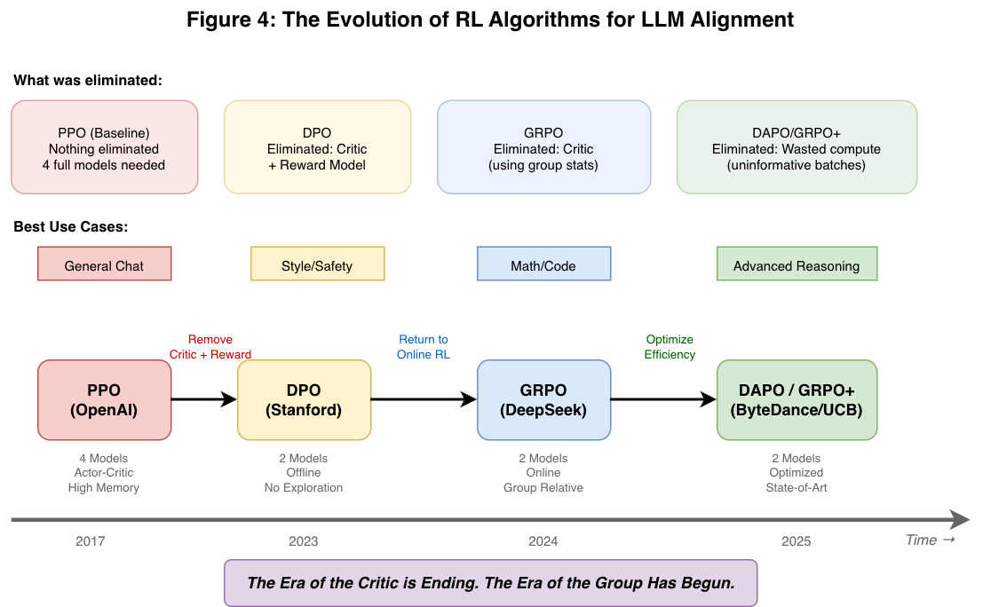
Figure 4: The evolution from PPO (2017) through DPO (2023), GRPO (2024), to DAPO/GRPO+/GDPO (2025-2026) shows a clear trend: eliminating proxies and unnecessary components while improving efficiency. Each algorithm eliminated something from its predecessor. DAPO optimizes single-objective efficiency, while GDPO solves the multi-objective problem that GRPO couldn’t handle.
When to Use Each Algorithm
| Scenario | Recommended Algorithm | Reason |
|---|---|---|
| Chat alignment (politeness, tone) | DPO | Efficient, stable, sufficient for style |
| Math reasoning (single objective) | DAPO | Best exploration, handles sparse rewards |
| Code generation | GRPO+ | KL-free allows radical policy shifts |
| Tool calling + Format constraints | GDPO | Multiple rewards with different scales |
| Agentic systems (safety + correctness) | GDPO | Prevents reward hacking across objectives |
| Any multi-reward optimization | GDPO | Per-reward normalization preserves all signals |
| Limited compute | DPO | No generation during training |
| Maximum single-objective performance | DAPO | State-of-the-art on reasoning benchmarks |
| Multi-objective + Efficiency | GDPO + DAPO tricks | Combine decoupled norm with dynamic sampling |
Future Directions
Process Reward Models (PRMs)
Current algorithms use Outcome Supervision (was the final answer correct?). The future lies in Process Supervision (was each reasoning step correct?).
Challenge: Labeling every step is expensive.
Solution: Algorithms like SCOPE automatically generate step-level rewards by:
- Translating reasoning into code
- Building prefix trees of solution paths
- Estimating step correctness from tree structure
Generative Reward Models (GenRM)
Instead of outputting a single score, GenRM outputs a “Chain of Thought” critique:
1 | Input: [Model's answer to a math problem] |
This provides richer signal than scalar rewards.
Self-Improving Loops
The next frontier: models that improve themselves through:
- Generate solutions
- Self-verify using learned verifier
- Update policy based on self-assessment
- Improve verifier based on new data
Conclusion
The Journey
The evolution of RL for LLMs follows a clear trajectory of eliminating proxies and solving specific problems:
| Era | Algorithm | What It Eliminated/Solved |
|---|---|---|
| 2017-2022 | PPO | Nothing (baseline Actor-Critic) |
| 2023 | DPO | Critic + Reward Model (offline) |
| 2024 | GRPO | Critic (using group statistics, online) |
| 2025 | DAPO | Gradient deadzones, entropy collapse |
| 2025 | GRPO+ | KL constraint (for radical policy shifts) |
| 2026 | GDPO | Reward signal collapse in multi-objective |
The Central Insights
Insight 1: The Critic is unnecessary for LLM training.
By comparing a model’s outputs against its own peers (Group Relative), we get:
- Unbiased baseline estimates
- 50% memory reduction
- Robustness to prompt difficulty
- Emergent reasoning behaviors (“Aha moments”)
Insight 2: Multi-objective optimization requires decoupled normalization.
When combining multiple reward signals:
- Sum-then-normalize causes reward signal collapse
- GDPO’s normalize-then-aggregate preserves all signals
- Critical for agentic systems with safety + correctness + format constraints
References
- John Schulman., et al, “Proximal Policy Optimization Algorithms,” 2017.
- Rafael Rafailov, et al, “Direct Preference Optimization: Your Language Model is Secretly a Reward Model,” 2024.
- Zhihong Shao, et al, “DeepSeekMath: Pushing the Limits of Mathematical Reasoning in Open Language Models,” 2024.
- DeepSeek-AI, et al. “DeepSeek-R1 incentivizes reasoning in LLMs through reinforcement learning,”, 2025.
- Qiying Yu, et al, “DAPO: An Open-Source LLM Reinforcement Learning System at Scale,” 2025.
- Shih-Yang Liu, et al, “GDPO: Group reward-Decoupled Normalization Policy Optimization for Multi-reward RL Optimization,” 2026.
- Ray Huang, et al, “Reinforcement Learning for Safe LLM Code Generation,” 2025.